At this site we consider the nature of earthquakes – how they fit within the framework of plate tectonics at a planetary scale and how they generate geologic features at the local scale, like the Stock Farm monocline; the slope you see in front of you. The 1906 earthquake ruptured nearly 300 miles of the San Andreas Fault, from San Juan Bautista in the south to Cape Mendocino in the north with an average fault offset of 10 feet. It provided the key evidence that established the connection of earthquakes with faulting. About 50 years later, the theory of plate tectonics established the role of the San Andreas in the global tectonic system and also the rate and sense of motion that must be accommodated across the Pacific North America plate boundary. While plate tectonics provides overall constraints on plate boundary deformation, detailed studies are required to discern the geologically active structures within that plate boundary and to quantify the hazards that they pose.

Elastic Rebound

The theory of plate tectonics holds that the Earth’s surface is comprised of a number of large plates that are thousands of kilometers in horizontal extent and approximately 100 km thick. These plates move relative to one another at about the rate that a fingernail grows and deform relatively little, except at their boundaries, where they slip past one another episodically in earthquakes. Plate-bounding faults, such as the San Andreas, are frictionally locked between earthquakes. During this locked phase, the Earth’s crust around plate boundaries slowly deforms elastically (it is doing so under your very feet as you read this). This elastic strain slowly accumulates until it raises the associated stress sufficiently to overcome the friction holding the fault in place. The fault then slips, the deformed crust “rebounds” like a broken spring, and suddenly releases the stored strain energy as seismic waves (Fig. 1).

Figure 1: Left panel demonstrates elastic rebound. As rock is stressed, it bends, storing elastic energy. Once the stress acting on the fault is sufficient to overcome friction, the fault slips and the stored energy is released in the form of earthquake waves (graphic from Earth by Tarbuck & Lutgens). Photograph on right shows fence in Marin County offset by slip in the 1906 earthquake.

This cycle of strain accumulation and release, referred to as elastic rebound, represents our fundamental understanding of how earthquakes work. “Elastic” in this context refers to the storage of energy in the crust as elastic (recoverable) strain. Deformation in the vicinity of the San Andreas Fault in the 1906 earthquake was carefully documented in the Lawson report, and this evidence convinced geologists that the elastic rebound hypothesis was correct. What was not at all clear at the time, however, was what caused the strain to accumulate in the first place. It was also not clear how quickly such strain might re-accumulate.

The Geomagnetic Polarity Time Scale

Figure 2 : Allan Cox (seated), Richard Doell (L), and Brent Dalrymple (R) at a gas mass spectrometer. This photo was taken sometime in the early 1960s. Image courtesy of Stanford School of Earth Sciences.

In the late 1950’s and 1960’s, a group of geologists at the US Geological Survey in Menlo Park was testing the notion that the Earth’s magnetic field periodically reverses it’s orientation, such that compasses that normally point toward the north at the Earth’s surface, would instead point towards the south. A group of scientists, consisting of Allan Cox (who subsequently joined the Stanford faculty and became Dean of the School of Earth Sciences), Brent Dalrymple, and Richard Doell (Fig. 2) systematically studied the orientation of the Earth’s magnetic field as it was preserved in volcanic rocks that cooled and acquired their magnetism shortly after they were erupted. This group demonstrated that reversals of the Earth’s magnetic field had occurred, and they were able to use radioactive isotopes to date the reversals. The result was a time scale based on variations in the Earth’s magnetic field, which later proved to be the “Rosetta Stone” for deciphering the pattern of magnetic anomalies on the sea floor. (Fig. 3)

Independently, scientists measuring magnetic field strength at sea during scientific oceanographic cruises found that the magnetic field they measured was strangely regular, with large stripes of similar magnetization. Fred Vine, Drummond Matthews, and Larry Morley realized this could be explained by a combination of sea floor magnetization as it was acquired during seafloor formation at mid-ocean ridges (Fig. 4), together with periodic reversals of the Earth’s magnetic field. This provided the key clue leading to the theory of plate tectonics. The distance of known magnetic anomalies from the mid-ocean ridges, together with the time at which they acquired their magnetization based on the geomagnetic polarity time scale, is used to determine the rate of plate motion. (Fig. 5) Thus by studying the seemingly unrelated field of geomagnetism, scientists were able to place quantitative constraints on the rates of plate motion, and hence the long-term rate of earthquakes at plate boundaries.

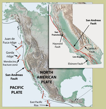
Earthquake Hazards in the Bay Area

Even before the emergence of the theory of plate tectonics, Mason Hill and Thomas Dibblee recognized that geologic features across the San Andreas Fault were offset by hundreds of miles. Estimates of the rate of motion based on geology and geodesy at the time ranged from about 5 to about 50 millimeters per year. Since then, global plate tectonic data indicates a somewhat higher rate of about 48 millimeters per year across this plate boundary. Not all of this motion is accommodated across the San Andreas Fault. Geodetic measurements of deformation, such as that based on ultra-precise GPS, confirms that offshore faults, other faults such as the Hayward fault in the East Bay, as well as faults as far east as Utah, accommodate the total plate motion. Nevertheless, plate tectonics provides the overall boundary condition on the system of plate boundary faults that is central to assessing the seismic hazard in the region. (Fig. 6).

Figure 6: Tectonic setting of the San Andreas Fault. Note the location of the Juan de Fuca and Gorda ridges (compare with Fig. 5).

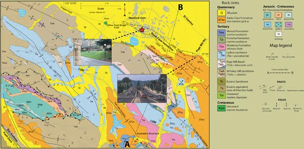
Figure 7: USGS figure showing significant Bay Area quakes. The 1906 earthquake relieved so much stress that there were few large quakes in the 20th century. As stress re-accumulates, large earth-quakes may be come commonplace, as they were in the late 1800s.

The identification of likely earthquake sources (active faults) and when earthquakes are likely to occur on them provides the foundation for assessing seismic hazard. The most recent synthesis of seismic hazards in the greater San Francisco Bay Area indicates that there is a 62% chance of at least one magnitude 6.7 or larger earthquake in the next 30 years (Fig. 7). This hazard is dominated by the major faults, such as the San Andreas, Hayward, and Rodgers Creek Faults, but the Bay Area is riven with faults, and there is always the possibility that the next big earthquake will occur on lesser-known or even currently unknown faults. Seismic hazard for the Stanford campus is dominated by the infamous San Andreas Fault, located about 5 miles southeast of campus (it crosses Page Mill Road at the Montebello Ridge Open Space Preserve). The San Andreas fault ruptured in the 1906 earthquake, of course, but prior to that it ruptured in 1838 in an earthquake of about magnitude 6.8 (Fig. 7) on the San Francisco Peninsula segment of the San Andreas. There are other faults in the area too. The slope in front of you is known as the Stock Farm Monocline. It is a deformational feature that is part of a fold and thrust belt that runs along the east side of the San Andreas Fault on the San Francisco Peninsula. (Figs. 8a-b)

Figure 8a: Geologic Map of Stanford Lands and Vicinity, mod. from Page, Ben M., 1993, Stanford Geologic Survey. Photos taken from the lower hinge of the monocline at Geocorner and Page Mill Road. Map courtesy of Stanford Geological Survey and R.G. Coleman; photos courtesy of R.L. Kovach.

Figure 8b: Generalized cross-section along line A-B on the geologic map.